A sleep spindle is a distinctive feature of electroencephalogram (EEG), which is characterized by progressively increased and gradually decreased 10~16 Hz oscillations [1]. It occurs during non-rapid eye movement (NREM) sleep and is temporally locked to the K-complex and vertex sharp wave [1]. In human EEG, sleep spindle is divided into two types, slow spindle (~12 Hz) in the frontal and fast spindle (~14 Hz) in parietal and central brain region [2,3,4,5,6]. Each type of spindle is affected differently by the same variables, such as age, lifestyle and medical history [7,8,9]. The differences between the two types of spindles suggest that each spindle is generated by a different mechanism. However, a different mechanism of spindle generation remains unclear due to lack of spatial information of sleep spindle propagation.

Previously we reported that regionally specific sleep spindles exist in rodents, as they do in human [10]. Also, we reported corticothalamic connection among cortex, thalamic nucleus, and reticular nucleus has distinctive patterns for anterior and posterior spindles. This suggests that each type of spindle generation in the mouse had a different generation mechanism. We believe that the knowledge of rodent spindle can be an effective channel to understand human spindle. However, for mice, the comprehensive method for neuroimaging and EEG topographic measure is limited due to the small size of mouse brain. Recently, we established the source localization technique [11] in mice with the developed high density EEG [12,13].

In this study, we have chosen to apply our novel neuroimage technique to each type of sleep spindle and visualized the dynamics of spindles.

We used the high density EEG data during spontaneous sleep which were collected, detected, and classified in our previous study [10]. Briefly, the high density EEG was obtained from polyimide-based microarray in freely moving mice [12,13]. The EEG was band-pass filtered and then the spindle detection algorithm was applied to the filtered signals based on a threshold method. The anterior and posterior spindles were classified based on K-mean clustering algorithm.

We used high density EEG signals of the anterior and posterior spindles, which were clustered based on K-means cluster analysis in our previous study [10]. The representative traces of anterior and posterior spindles were presented in Fig. 2. In each panel, the left column contains the raw signals and the right column contains the filtered signals. The topographies of total power of the corresponding anterior and posterior spindles overlay the cortical surface of mouse brain in (C) and (D), respectively.

We followed the procedures for the dipole source localizations described in our previous work (Fig. 1 in [11]). Briefly, the boundary element model for the mouse brain was built based on mouse MRI to compute the leadfield matrix. Four different source localization algorithms (minimum norm [16], LORETA [17,18], sLORETA [19] and eLORETA [20]) were applied and their performance was compared. As a demonstration, the posterior spindle shown in Fig. 2B was applied and the axial and coronal view of its estimated source distributions are shown in Fig. 3A and 3B, respectively. While the spatial distributions of horizontal axis were similar for all algorithms, the spatial distributions of vertical axis were different depending on the algorithms. The LORETA or modified LORETA algorithms estimated the source deeper compared to MN. In our previous study based on optogenetic stimulation, the LORETA algorithm estimated the source deeper than the real source position [11]. On the other hand, the minimum norm algorithm estimated the sources successfully confined to the cortex.

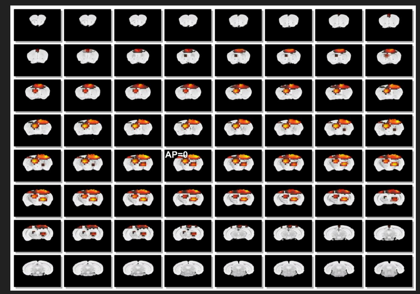
The advantage of source localization is in the ability to visualize the propagation of potential sources generating the cortical potentials. Therefore, we employed the weighted norm algorithm to sleep spindles to visualize the propagation of cortical sources as time passes and presented in cine mode for anterior and posterior sleep spindles in Fig. 4 and Fig. 5, respectively. The cine mode presentation shows the spatio-temporal patterns of spindle evolution over time. For example, the sources of posterior spindles were confined to the posterior regions, but their positions fluctuated within the posterior cortex. A movie with high temporal resolution showed that the first slow wave of spindles was generated in the somatosensory cortex and propagated to the motor cortex, but the last slow wave of spindle was generated in the motor cortex and then propagated to the somatosensory cortex, showing complex patterns of onset and propagation of sleep spindles. This visualization confirms that the spindles are dynamical phenomena rather than an event of one entity.

In this study, we evaluated the performance of four different algorithms for source localization of spindles. The flow direction of source cluster was similar, but LORETA or modified LORETA algorithms overshoot the depth of source. Generally, cortical dipole was regarded as the source of EEG [21]. Many studies have suggested that the rodent EEG has identical characteristics as the human EEG [10,22]. Also, an electrode with the impedance of several hundred ohms can only measure the signal in 250 µm [23]. Additionally, we used common average reference. This method cancels out the signal from deep brain region. Therefore, the subcortical source was not reasonable. One of the major possible sources of error is the electrode position. All our electrodes were located above the upper surface. Therefore, depth of source localization solution could be biased. The MN is used to analyze evoked responses that involve wide-spread neuronal activation over time. In addition, MN tends to reconstruct sources that are superficial [24,25]. Therefore, we recommended that MN method is suitable for mouse brain.

As a comparable tool for noninvasive functional brain mapping, functional magnetic resonance imaging (fMRI) has been used in human brain mapping. However, the fMRI is based on blood oxygen level dependenet level rather than neural activity like EEG. EEG is the sum of synchronized post-synaptic activities, whereas BOLD response represents the change of hemodynamics that was related to the total synaptic activity. Additionally, EEG and the BOLD signal were caused by different cellular populations [26]. Previous research shows that average distance between local field potential and centroid of functional MRI was 1 cm in half of the monkey sensory cortex recording [27]. As previously mentioned, EEG is more related to functional neural activity and have a better temporal resolution to understand fast brain dynamics. Besides, the temporal resolution of fMRI is inappropriate to trace the fast activities like sleep spindles.

In sum, this study employed the equivalent dipole source estimation method in visualizing the sleep spindles in mouse brain. By applying source localization method, we have shown that the anterior and posterior spindles do not have identical functional brain mapping and temporal change of spindle dynamics. Our result suggests the possibility of the minimally invasive functional approach of the spindle network analysis. Also, our approach may advance our understanding for the functional study of cortical network in mice.

References

- De Gennaro L, Ferrara M. Sleep spindles: an overview. Sleep Med Rev 2003;7:423-440.
- Anderer P, Klösch G, Gruber G, Trenker E, Pascual-Marqui RD, Zeitlhofer J, Barbanoj MJ, Rappelsberger P, Saletu B. Low-resolution brain electromagnetic tomography revealed simultaneously active frontal and parietal sleep spindle sources in the human cortex. Neuroscience 2001;103:581-592.
- Jobert M, Poiseau E, Jähnig P, Schulz H, Kubicki S. Topographical analysis of sleep spindle activity. Neuropsychobiology 1992;26:210-217.
- Schabus M, Dang-Vu TT, Albouy G, Balteau E, Boly M, Carrier J, Darsaud A, Degueldre C, Desseilles M, Gais S, Phillips C, Rauchs G, Schnakers C, Sterpenich V, Vandewalle G, Luxen A, Maquet P. Hemodynamic cerebral correlates of sleep spindles during human non-rapid eye movement sleep. Proc Natl Acad Sci U S A 2007;104:13164-13169.
- Werth E, Achermann P, Dijk DJ, Borbély AA. Spindle frequency activity in the sleep EEG: individual differences and topographic distribution. Electroencephalogr Clin Neurophysiol 1997;103:535-542.
- Zygierewicz J, Blinowska KJ, Durka PJ, Szelenberger W, Niemcewicz S, Androsiuk W. High resolution study of sleep spindles. Clin Neurophysiol 1999;110:2136-2147.
- Ayoub A, Aumann D, Hörschelmann A, Kouchekmanesch A, Paul P, Born J, Marshall L. Differential effects on fast and slow spindle activity, and the sleep slow oscillation in humans with carbamazepine and flunarizine to antagonize voltage-dependent Na+ and Ca2+ channel activity. Sleep 2013;36:905-911.
- Schönwald SV, Carvalho DZ, de Santa-Helena EL, Lemke N, Gerhardt GJ. Topography-specific spindle frequency changes in obstructive sleep apnea. BMC Neurosci 2012;13:89.
- Tamaki M, Matsuoka T, Nittono H, Hori T. Fast sleep spindle (13–15 hz) activity correlates with sleep-dependent improvement in visuomotor performance. Sleep 2008;31:204-211.
- Kim D, Hwang E, Lee M, Sung H, Choi JH. Characterization of topographically specific sleep spindles in mice. Sleep 2015;38:85-96.
- Lee C, Oostenveld R, Lee SH, Kim LH, Sung H, Choi JH. Dipole source localization of mouse electroencephalogram using the fieldtrip toolbox. PLoS One 2013;8:e79442.
- Choi JH, Koch KP, Poppendieck W, Lee M, Shin HS. High resolution electroencephalography in freely moving mice. J Neurophysiol 2010;104:1825-1834.
- Lee M, Kim D, Shin HS, Sung HG, Choi JH. High-density EEG recordings of the freely moving mice using polyimide-based microelectrode. J Vis Exp 2011.
- Ma Y, Hof PR, Grant SC, Blackband SJ, Bennett R, Slatest L, McGuigan MD, Benveniste H. A three-dimensional digital atlas database of the adult C57BL/6J mouse brain by magnetic resonance microscopy. Neuroscience 2005;135:1203-1215.
- Ma Y, Smith D, Hof PR, Foerster B, Hamilton S, Blackband SJ, Yu M, Benveniste H. In vivo 3D digital atlas database of the adult C57BL/6J mouse brain by magnetic resonance microscopy. Front Neuroanat 2008;2:1.
- Fuchs M, Wagner M, Köhler T, Wischmann HA. Linear and nonlinear current density reconstructions. J Clin Neurophysiol 1999;16:267-295.
- Pascual-Marqui RD. LORETA in 3D solution space. ISBET Newsl 1995;6:22-28.
- Wagner M, Fuchs M, Wischmann HA, Drenckhahn R, Köhler T. Smooth reconstruction of cortical sources from EEG or MEG recordings. Neuroimage 1996;3:S168.
- Pascual-Marqui RD. Standardized low-resolution brain electromagnetic tomography (sLORETA): technical details. Methods Find Exp Clin Pharmacol 2002;24:5-12.
- Pascual-Marqui RD, Lehmann D, Koukkou M, Kochi K, Anderer P, Saletu B, Tanaka H, Hirata K, John ER, Prichep L, Biscay-Lirio R, Kinoshita T. Assessing interactions in the brain with exact low-resolution electromagnetic tomography. Philos Trans A Math Phys Eng Sci 2011;369:3768-3784.
- Niedermeyer E, da Silva FL. Electroencephalography: basic principles, clinical applications, and related fields. 5th ed. Philadelphia, PA: Lippincott Williams & Wilkins, 2005.
- Kim B, Kocsis B, Hwang E, Kim Y, Strecker RE, McCarley RW, Choi JH. Differential modulation of global and local neural oscillations in REM sleep by homeostatic sleep regulation. Proc Natl Acad Sci U S A 2017;114:E1727-E1736.
- Kajikawa Y, Schroeder CE. How local is the local field potential?. Neuron 2011;72:847-858.
- Dale AM, Liu AK, Fischl BR, Buckner RL, Belliveau JW, Lewine JD, Halgren E. Dynamic statistical parametric mapping: combining fMRI and MEG for high-resolution imaging of cortical activity. Neuron 2000;26:55-67.
- Hämäläinen MS, Ilmoniemi RJ. Interpreting magnetic fields of the brain: minimum norm estimates. Med Biol Eng Comput 1994;32:35-42.
- Nunez PL, Silberstein RB. On the relationship of synaptic activity to macroscopic measurements: does co-registration of EEG with fMRI make sense?. Brain Topogr 2000;13:79-96.
- Disbrow EA, Slutsky DA, Roberts TP, Krubitzer LA. Functional MRI at 1.5 tesla: a comparison of the blood oxygenation level-dependent signal and electrophysiology. Proc Natl Acad Sci U S A 2000;97:9718-9723.